夏の自由研究連載 2024 の 2 日目です。
Slack のカスタム絵文字を AI で遊びました。
前書き 夏の自由研究連載 2023 の「Sentence-Transformers を使って YouTube 動画のセリフを検索する 」では、テキストのセマンティック検索や文字資料に対して Q&A に注目してデモしました。しかし Sentence-Transformers は、テキストだけではなく、画像や音声など異なる情報の組み合わせ、いわゆる マルチモーダル(multi-modal) AI のモデルです。
そのため、同一のモデルで、文字と画像を意味的な関連性を利用して、同一のベクトル空間に埋め込み(Embedding)することで、数学の計算(ベクトルの cosine 距離など)で近似度の評価が実現できます。
テキストと画像を検索のインプットとアウトプットの組み合わせで、以下の応用場面を例として挙げられます。
今回は、前回割愛した画像に関するセマンティック検索について実践します。入力として Slack のカスタム絵文字を扱います。
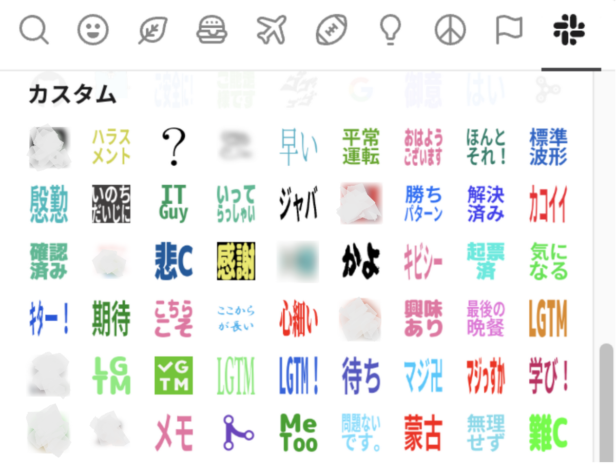
仕事上でもよく使われる Slack では、ユーザが小さな画像もしくは画像化した文字をカスタム絵文字として自由にアップロードできます。ドアが開けっぱなしに思えますが、現在我々使っている Slack ワークスペースに、5000 個以上のカスタム絵文字が存在し、また日々増え続けており、重複や類似の絵文字がたくさん存在します。
また、アップロード時に絵文字の名称を指定する必要がありますが、一意であれば良いので少し雑な命名も多いです。名前での検索しても、使いたい絵文字はなかなか見つからないこともしばしばです。
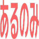
例えば、↓ 最初のaから始まる絵文字を紹介します。具体例を見れば雰囲気がわかると思います。
それになんとかしたい気持ちで、絵文字の重複検知、便利に使いたい絵文字を意味で検索できるために、セマンティック検索の AI 技術を応用してみました。
データの準備 まずは、ローカルでデータを扱うように、Slack カスタム絵文字をクローリングでダウンロードします。
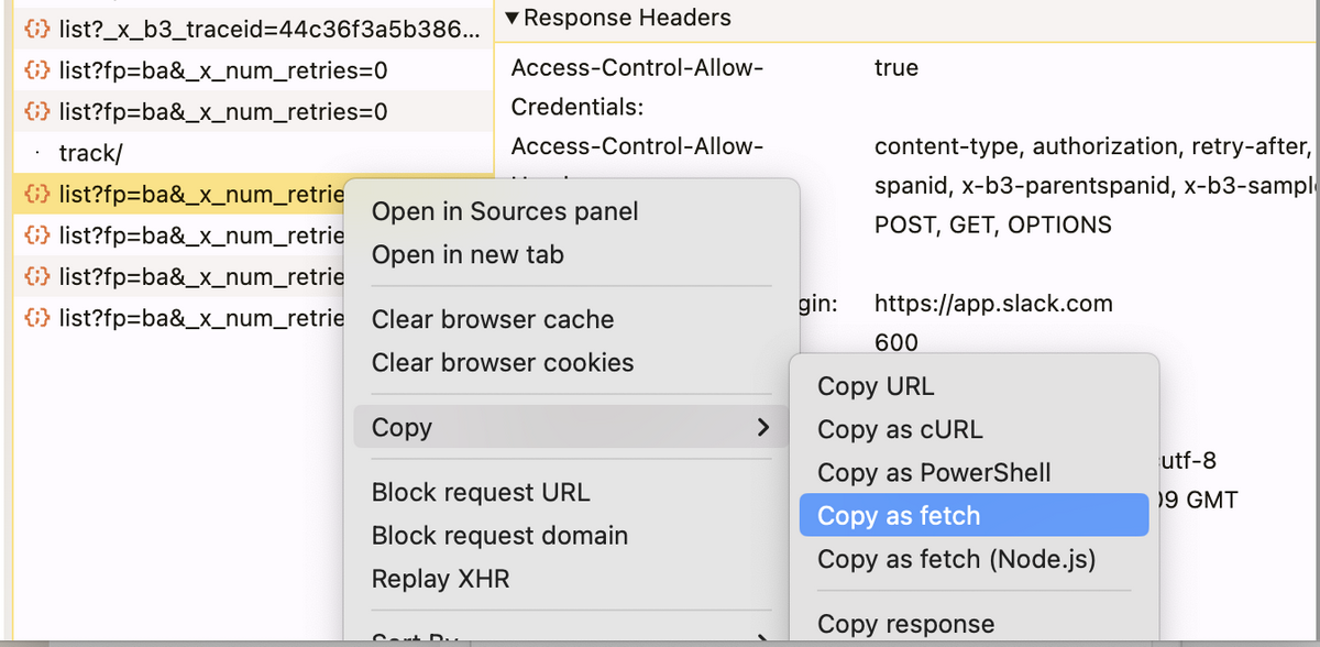
絵文字を表示するときブラウザから投げだした API を fetch 句で拾って、以下になります。
fetch ("https://edgeapi.slack.com/cache/xxxx/emojis/list?fp=ba&_x_num_retries=0" , { "headers" : { "content-type" : "text/plain;charset=UTF-8" , ... }, "referrerPolicy" : "no-referrer" , "body" : "{\"token\":\"xxxx\",\"count\":100,\"marker\":\"compliance_warning_コンプラ\",\"enterprise_token\":\"xxxx\"}" , "method" : "POST" , "mode" : "cors" , "credentials" : "include" });
レスポンスがページネーションされて、100 件ずつ取っていることが分かりました。
その挙動をシミュレートする Python のスクリプトを作って、全量の絵文字名と URL を yaml ファイルに保存します。
from requests import Sessionimport yamllist_emojis_url = ( "https://edgeapi.slack.com/cache/xxxx/emojis/list?fp=ba&_x_num_retries=0" ) cookie_string = '<ログイン処理が面倒なので、ブラウザのクッキー情報を引っ張ってくる>' token = "xxxx" s = Session() for cookie in cookie_string.split("; " ): name, value = cookie.split("=" , 1 ) s.cookies.set (name, value) marker = "_doing" while True : json_data = { "token" : token, "enterprise_token" : token, "count" : 100 , "marker" : marker, } response = s.post(url=list_emojis_url, json=json_data).json() with open ("results.yaml" , "a" ) as f: yaml.dump(response["results" ], f) marker = response.get("next_marker" ) if marker is None : break
保存した yaml ファイルは以下のような形になります。
- name: _doing
  updated: 1642723962
  value: https://emoji.slack-edge.com/T01310927L1/_doing/15ac6e3e64ce0764.png
- name: -sherlock-holmes-costume
  updated: 1720678172
  value: https://emoji.slack-edge.com/T01310927L1/-sherlock-holmes-costume/0d46d4d059e8f066.png
- ...
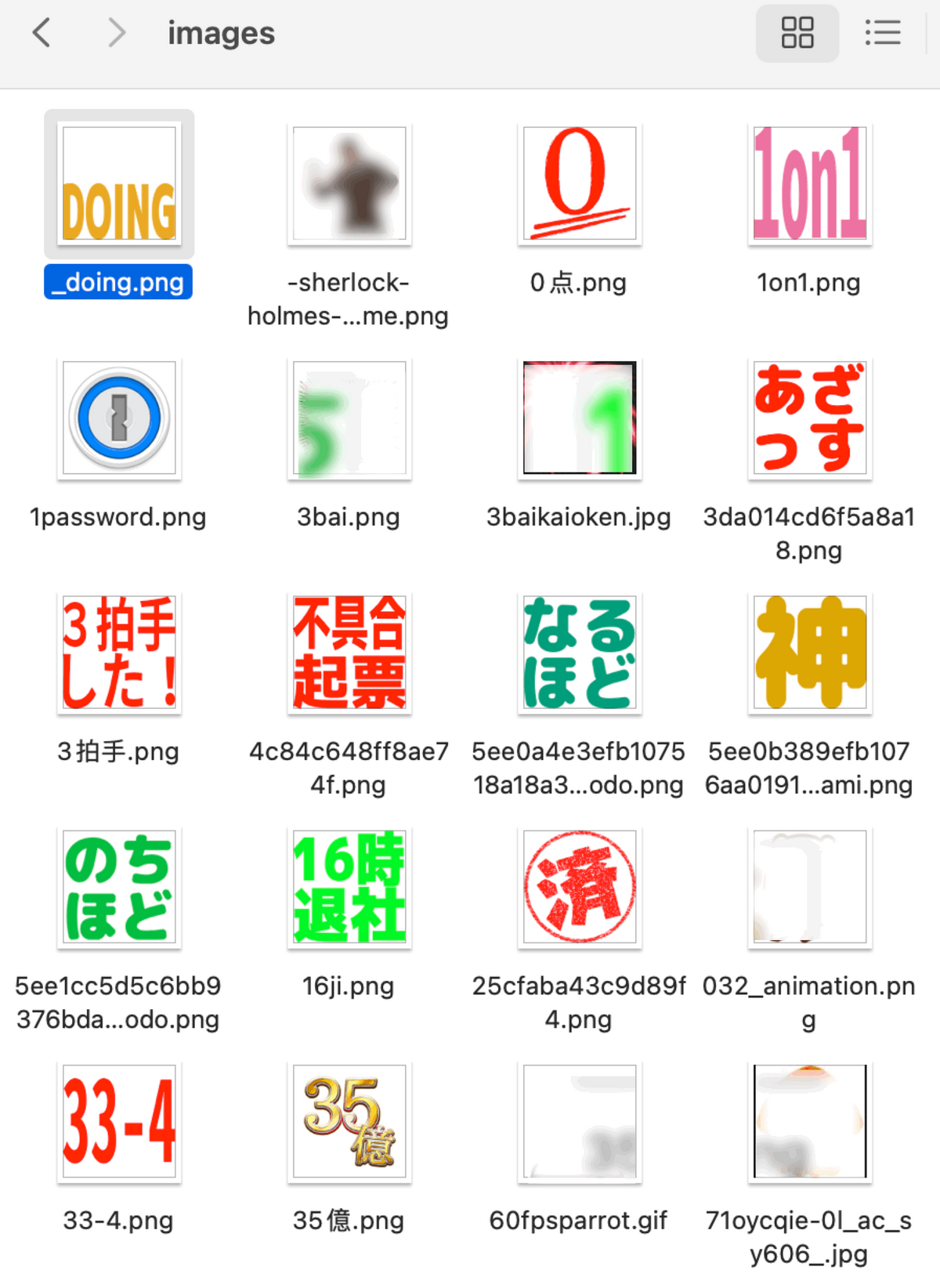
yaml に記載してあった value を URL として、name を保存先のファイル(拡張子は URL を尊重する)として、ローカルにダウンロードします。
import osimport requestsimport yamldef read_yaml_result (filename ): with open (filename) as input_data: return yaml.safe_load(input_data) def download_image (file_path, url ): try : response = requests.get(url) response.raise_for_status() with open (file_path, "wb" ) as file: file.write(response.content) print (f"Downloaded {file_path} " ) except requests.exceptions.RequestException as e: print (f"Failed to download {name} : {e} " ) if __name__ == "__main__" : input_file_name = "results.yaml" output_directory = "images" os.makedirs(output_directory, exist_ok=True ) skip = True for item in read_yaml_result(input_file_name): name = item["name" ] url = item["value" ] if skip and name == "simple_smile" : skip = False if skip: continue _, ext = os.path.splitext(url) file_path = os.path.join(output_directory, f"{name} {ext} " ) download_image(file_path, url)
ファイルを正しくダウンロードできたことが確認できました。
画像データのベクトル化 Sentence-Transformers のこのページ をベースとして参考して、画像をベクトルに Embedding しておきます。
※ ファイル数が多すぎますので、デモ用で 1000 ファイルのみ処理します。
import osfrom PIL import Imagefrom sentence_transformers import SentenceTransformerimages_dir = "images" max_images = 1000 model = SentenceTransformer("clip-ViT-B-32" ) image_files = [os.path.join(images_dir, file) for file in os.listdir(images_dir)][ :max_images ] images = [] image_labels = [] for image_file in image_files: images.append(Image.open (image_file)) base, ext = os.path.splitext(os.path.basename(image_file)) image_labels.append(base) img_emb = model.encode(images) print (img_emb)print (img_emb.shape)
実行結果です。
$ python3 visualize.py
[[ 0.3558431  -0.4127885  -0.38162816 ...  0.8868538  -0.24081565
   0.11687451]
 [ 0.35159412 -0.22937642 -0.28752807 ...  0.7736969  -0.5258111
   0.40994892]
 [ 0.23833637 -0.2584821  -0.3712055  ...  0.89749026  0.03570646
  -0.2068485 ]
 ...
 [ 0.17339917 -0.16685665  0.13446489 ...  0.87421316 -0.18107425
   0.39892197]
 [ 0.17150897  0.18003528 -0.40643013 ...  0.9075323  -0.35873666
   0.00515198]
 [-0.26825747 -0.1587921   0.04072791 ...  0.9843429  -0.40589246
   0.00923938]]
(1000, 512)
“clip-ViT-B-32” モデルで、1000 個の画像データをそれぞれ 512 次元のベクトルに変換できました。
そのベクトルを使って、画像間の距離計算、分類、検索など、色々なことができます。
その多次元のベクトルを主要要素を抽出して 2 次元に圧縮して、画面上に描画する方法を ChatGPT 先生に教えてもらいました。
たくさんオプションが教えられていますが、1 個目の TSNE でも良いでしょう。
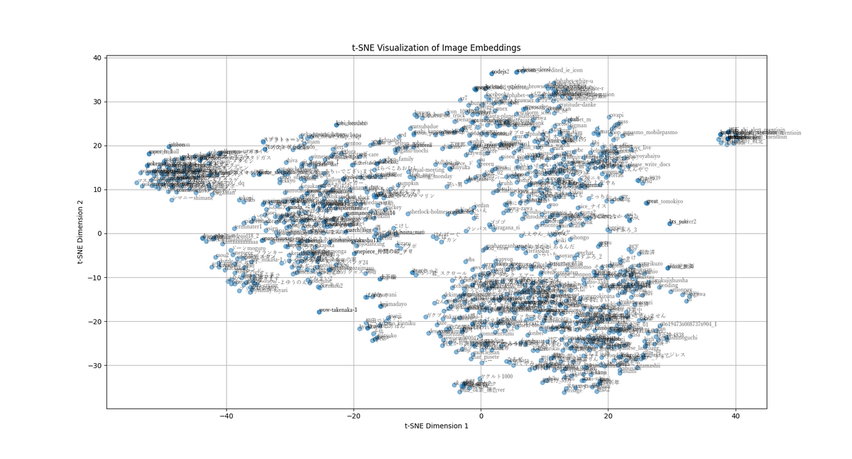
早速描画してみましょう。
import matplotlib.pyplot as pltfrom sklearn.manifold import TSNEperplexity_value = min (30 , len (img_emb) - 1 ) tsne = TSNE(n_components=2 , perplexity=perplexity_value, random_state=0 ) reduced_embeddings = tsne.fit_transform(img_emb) num_clusters = 5 kmeans = KMeans(n_clusters=num_clusters, random_state=0 ) cluster_labels = kmeans.fit_predict(reduced_embeddings) plt.figure(figsize=(15 , 9 )) plt.scatter(reduced_embeddings[:, 0 ], reduced_embeddings[:, 1 ], alpha=0.5 ) for i, label in enumerate (image_labels): plt.text( reduced_embeddings[i, 0 ], reduced_embeddings[i, 1 ], label, fontsize=8 , alpha=0.6 , fontname="YuMincho" , ) plt.title("t-SNE Visualization of Image Embeddings" ) plt.xlabel("t-SNE Dimension 1" ) plt.ylabel("t-SNE Dimension 2" ) plt.grid(True ) plt.show()
うんん、なるほどの感じですね。多すぎてみにくいですね。
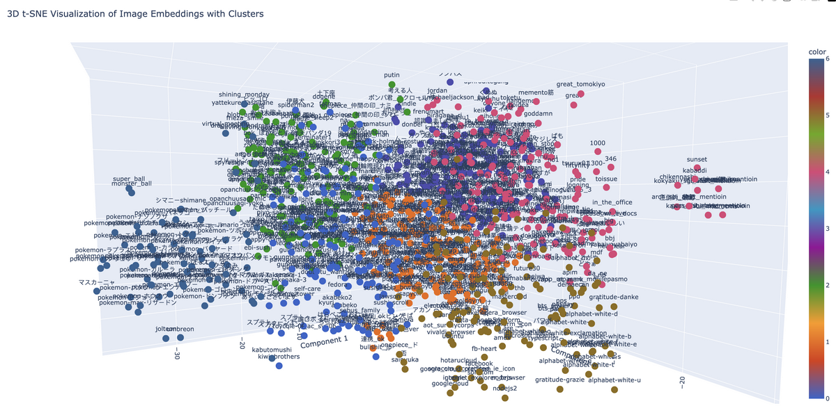
空間的分類クラスタ plotly を利用して、3D でも描画しようと思います。
from sklearn.cluster import KMeansimport plotly.express as pxnum_clusters = 7 kmeans = KMeans(n_clusters=num_clusters, random_state=0 ) cluster_labels = kmeans.fit_predict(reduced_embeddings) fig = px.scatter_3d( x=reduced_embeddings[:, 0 ], y=reduced_embeddings[:, 1 ], z=reduced_embeddings[:, 2 ], color=cluster_labels, text=image_labels, labels={"x" : "Component 1" , "y" : "Component 2" , "z" : "Component 3" }, title="3D t-SNE Visualization of Image Embeddings with Clusters" , color_continuous_scale=px.colors.qualitative.G10, )
さっきのポケモンシリーズのクラスタを左になるように回転しておきました。
結果はブラウザ上で閲覧しています。ズームや回転の操作はこんな感じです。
ファイル名の表示を隠して、細かく 20 分類(num_clusters = 20)にしてみたら、こんな感じです。
画像で画像を検索 近似画像を検索する手法は、データと同じくクエリ用の画像の特徴ベクトルを計算(Embedding)し、既存データのベクトルの類似度(今回のモデルは cosine 距離)を計算し、類似度高い順で結果を取得するという流れです。
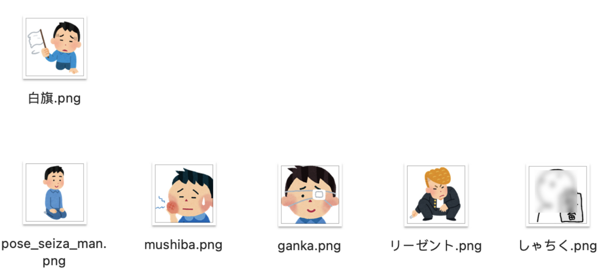
query_emb = model.encode(Image.open ("images/白旗.png" )) similarities = model.similarity(query_emb, img_emb).reshape((-1 ,)) k = 5 top_k_indices = reversed (np.argsort(similarities)[-k:]) top_k_similarities = similarities[top_k_indices] for i, (index, score) in enumerate (zip (top_k_indices, top_k_similarities)): print ( f"Rank {i + 1 } : Image Name: {image_files[index]} , Similarity Score {score:.4 f} " )
結果例 1
クエリ画像:images/白旗.png
ヒットした Top5 の画像:
Rank 1: Image Name: images/pose_seiza_man.png, Similarity Score 0.8798
Rank 2: Image Name: images/mushiba.png, Similarity Score 0.8741
Rank 3: Image Name: images/ganka.png, Similarity Score 0.8697
Rank 4: Image Name: images/リーゼント.png, Similarity Score 0.8454
Rank 5: Image Name: images/しゃちく.png, Similarity Score 0.8415
今回のクエリ画像は、全体の 5000+の画像から選択した 1000 件に含まれていないため、Top1 がクエリ画像自身をヒットしていないです。
上位の 3 個のヒットは同一キャラクタのことが分かりますね。
結果例 2
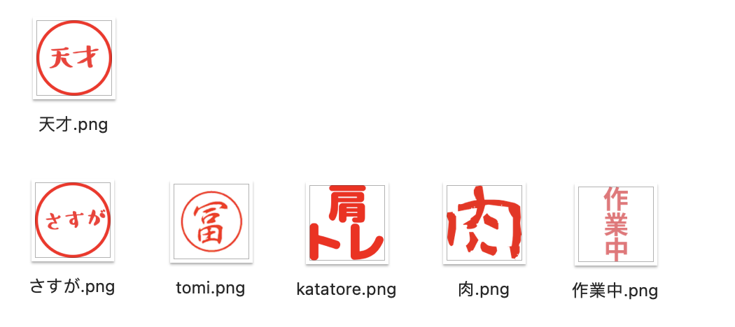
クエリ画像:images/天才.png
ヒットした Top5 の画像:
Rank 1: Image Name: images/さすが.png, Similarity Score 0.9758
Rank 2: Image Name: images/tomi.png, Similarity Score 0.9647
Rank 3: Image Name: images/katatore.png, Similarity Score 0.9639
Rank 4: Image Name: images/肉.png, Similarity Score 0.9570
Rank 5: Image Name: images/作業中.png, Similarity Score 0.9537
近似度みんな高い(0.95 以上)です。画像の中の文字の意味が理解していない様子です。
印鑑系丸くて赤い文字が特徴でしょう。ただ、最後の「作業中」は丸くもないですけど。
肩トレの「レ」や「肉」文字の外側、ちょっと丸くなっている感が見えているのでしょう。
文字で画像を検索 上記画像から画像の検索と似たように、同じモデルで、文字列も同様な Embedding 処理ができます。
ちなみに、日本語でも検索できるようにしたい場合は、多言語対応の“clip-ViT-B-32-multilingual-v1” モデルを使ったほうがいいそうです。
ただ、画像の Embedding は“clip-ViT-B-32” のままを使用するのが正しいです。
model2 = SentenceTransformer("clip-ViT-B-32-multilingual-v1" ) query_emb = model2.encode("ポケモンボール" ) similarities = model.similarity(query_emb, img_emb).reshape((-1 ,))
ただ、文字が画像の中身を抽象的な名称では、あまりヒットしなく、画像の形状や色、物体の表現のほうがヒットしやすいです。
例えば、以下具体の結果例:
クエリ文字: "ポケモンボール"
Rank 1: Image Name: images/おっとっと.png, Similarity Score 0.2725
Rank 2: Image Name: images/images.png, Similarity Score 0.2725
Rank 3: Image Name: images/anpn_アンパンチ.png, Similarity Score 0.2682
Rank 4: Image Name: images/piyo_mushin.png, Similarity Score 0.2675
Rank 5: Image Name: images/piyo-mushin.png, Similarity Score 0.2675
以下の色や形状の表現ならヒットします(ただ、近似度 0.26 は高くないです)。
クエリ文字: "上は赤、下は白、球体"
Rank 1: Image Name: images/monster_ball.png, Similarity Score 0.2619
Rank 2: Image Name: images/ポンパ君_スクロール.gif, Similarity Score 0.2521
Rank 3: Image Name: images/redmine.png, Similarity Score 0.2512
Rank 4: Image Name: images/alert.gif, Similarity Score 0.2495
Rank 5: Image Name: images/spiderman2.jpg, Similarity Score 0.2492
ただし、下記の特定な名称では、またヒットします。
クエリ文字: "ビーチボール"
Rank 1: Image Name: images/monster_ball.png, Similarity Score 0.2570
Rank 2: Image Name: images/おっとっと.png, Similarity Score 0.2544
Rank 3: Image Name: images/images.png, Similarity Score 0.2544
Rank 4: Image Name: images/panda_マスク.png, Similarity Score 0.2543
Rank 5: Image Name: images/piyo_mushin.png, Similarity Score 0.2541
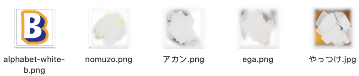
最後に、みんなが大好きな「ビール」でテストしてみましょう。
クエリ文字: "ビール"
Rank 1: Image Name: images/alphabet-white-b.png, Similarity Score 0.2633
Rank 2: Image Name: images/nomuzo.png, Similarity Score 0.2517
Rank 3: Image Name: images/アカン.png, Similarity Score 0.2511
Rank 4: Image Name: images/ega.png, Similarity Score 0.2438
Rank 5: Image Name: images/やっつけ.jpg, Similarity Score 0.2433
また笑い話になりますが、トップでヒットしたのは「ビー」の部分でした!
また、今回のデモでは、1 個のクエリベクトルに対して、全データ(1000 個)のベクトルとの近似度(Cosine Similarity)が計算して、ソートをかけてしまいましたが、もし事前にインデックスを立てたり、近似な結果も許されたりする場合、k-近傍法(k-NN)のもっと効率的なアルゴリズムもあります(割愛)
まとめ 2023年の記事の続きとして、事前訓練された(pre-trained)マルチモーダル(multi-modal)の AI モデルを使った画像処理を実践してみました。
Slack のカスタム絵文字のデータを利用して、関連性によってクラスタ化して、可視化グラフを書いてみました。
また、セマンティック検索について、検証の結果は指標化までできていませんが、直感的に、
「画像 → 画像」の検索は、なんとなく精度が悪くなく
「文字 → 画像」の検索はすぐには実用化とはちょっと微妙
そして、近似データや重複データの検知や排除する手法として、他の領域へも応用できそうだと思います。